By Ken Gregory © November 13, 2017
Many people are concerned that anthropogenic greenhouse gas emissions, primarily carbon dioxide (CO2), will increase temperatures and cause increasing damages from more intense and frequent storms and hurricanes. There have been numerous stories in the media falsely claiming that rising temperatures cause hurricanes to be “more horrifying”. There is little to no evidence that increasing temperatures have in the past or will in the future cause more intense storms and hurricanes.
Rising temperatures are expected to reduce the polar to tropics temperature gradient, which powers extra-tropical storms, so warming should reduce their intensity; whereas, tropical hurricanes are powered by the temperature difference between the top-of-clouds and the sea surface. The amount of wind shear, being the change in wind velocity with altitude, also plays a large role in hurricane formation and intensity. There was an active hurricane season this year due to low wind shear over the tropical Atlantic Ocean which favors hurricane formation. Hurricane Harvey on August 26, 2017 ended an 11-year, 10-month lack of major (Cat 3+) hurricanes making USA landfall, the longest period in history. The previous major hurricane making USA landfall was Wilma in October 24, 2005. Increasing temperatures are expected to slightly decrease the temperature difference between the surface and cloud top, as the cloud top warms more than the surface, which helps to reduce the intensity of hurricanes. The overall temperature plays a small role in increasing hurricane intensity, but higher temperatures likely causes more rainfall.
A fine mesh climate simulation predicts that a 1 °C temperature increase would decrease the global frequency of tropical cyclones by 17% and would increase the ratio of intense tropic cyclones by 5%. The model predicts rainfall would increase by 9% (Yamada et al 2017). However, computer models are notoriously bad at simulating the atmospheric temperature profile, so the simulated results may be misleading.
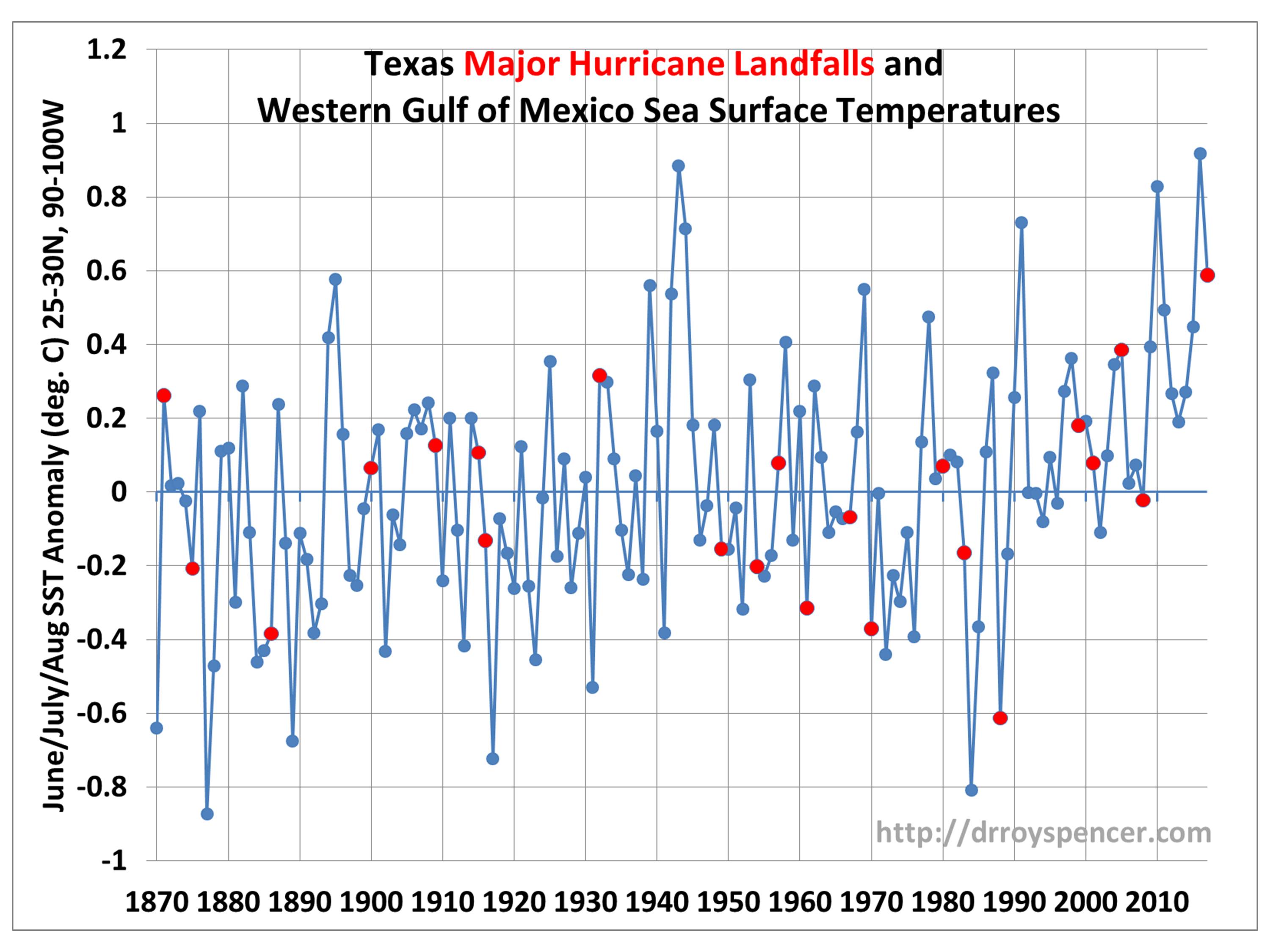
Dr. Spencer published a graph here showing the sea surface temperature of the western Gulf of Mexico of major hurricane strikes in Texas since 1870, presented as Figure 1. The red dots on the graph represent the years of major hurricane strikes in Texas. The graph shows that major hurricanes are just as likely when sea temperatures are below average as when they are above average. There were 11 major hurricanes with above average sea surface temperatures and 11 with below average sea surface temperatures. Spencer writes, “major hurricanes don’t really care whether the Gulf is above average or below average in temperature”. See here.
Dr. Ryan Maue produces graphical records of tropical hurricane frequency and accumulated energy. The accumulated cyclone energy (ACE) index is a running 24 month of the cyclone energy, thereby combining the frequency and intensity of all cyclones with maximum wind speeds exceeding 64 knots.
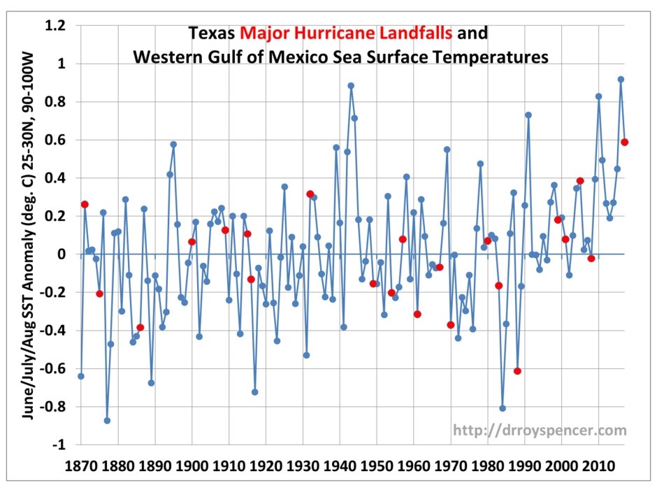
Figure 1.

Figure 2.
Figure 2 is a graph of the global tropical ACE indicates significant decadal variability but no significant trend. See the hurricane frequency graph here.
The FUND integrated assessment model is the world’s most detailed model designed to predict the economic and social effects of climate change due to greenhouse gas emissions. It estimates the costs and benefits of CO2 emissions for 16 regions and for the global total by 15 impact components.
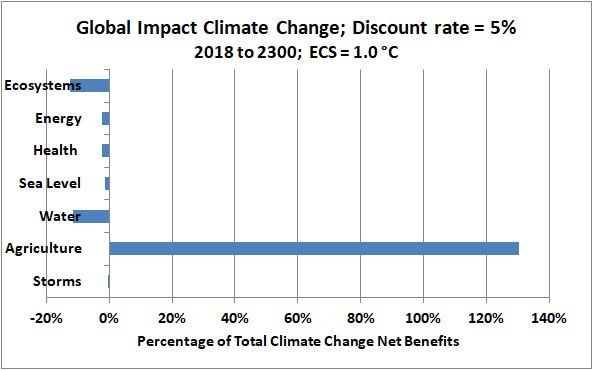
Figure 3.
The biggest factor in determining the impact of emissions is the sensitivity of the climate to changes in the concentration of CO2 in the atmosphere. Nick Lewis and Judith Curry published an empirical study of the climate sensitivity, and Nick Lewis updated it using updates aerosol forcing estimates. Their best estimate of the equilibrium climate sensitivity (ECS), without removing the effects of urban warming on the temperature record and the millennium warming cycle, is 1.45 °C per a doubling of the CO2 concentration. Correcting this estimate by the urban warming effect and the millennium warming cycle gives a best estimate of 1.02 °C. Using a 1.0 °C estimate of ECS, the FUND model shows the damages from storms, including extra-tropical storms and tropical hurricanes, is 0.54% of the net present value benefits for the period 2018 to 2300, using a discount rate of 5%, as indicated in the bar graph of Figure 3. The bar representing the damages from storms is just barely visible. The damages from storms is only 0.41% of the benefits from agriculture. Agriculture benefit from both warming and the CO2 fertilization effect, as CO2 is plant food.
Figure 4 shows seven grouping of welfare impact changes from 1950 per global domestic product (GDP) as calculated by the FUND model, assuming an ECS of 1.0 °C for the period 1950 to 2200. ECS is the temperature change in response to a doubling of atmospheric CO2 after waiting for the oceans to reach temperature equilibrium, which can take thousands of years.

Figure 4.
The GDP is the sum of all countries’ gross domestic products, or the world total income. Comparing the damages to total income allows us to see that projected storm damages due to our emissions are insignificant. The blue ‘Storms’ curve is the line just above the purple ‘Sea Level’ curve, which at this scale, is almost indistinguishable from 0%. You have to look very closely at the graph to see the two curves. FUND calculates, assuming an ECS of 1.0 °C, that the global storm damages change from 1950 to the year 2100 are 0.0046% of GDP, which is very insignificant. All the media hype about CO2 emissions making storms more horrible is misplaced. The graph of global welfare per GDP by component must be understood in context with the assumed CO2 emissions. The default emissions in FUND assumes CO2 emission per year increases from 30.4 gigatonnes CO2 (GtCO2) in 2017 to a maximum of 95.8 GtCO2 in 2115, which is a huge increase considering that there was no increase in CO2 emissions over the last three years of data to 2016.
If you are inclined to believe climate sensitivity estimates from climate models that do not work, rather than estimates from empirical measurements, then you might want to know the storm damages change as a percentage of GDP calculated by FUND using an ECS of 3.0 °C for a doubling of atmospheric CO2. The Intergovernmental Panel on Climate Change gives a central estimate of ECS of 3 .0 °C by assuming all warming is caused by greenhouse gas emission and that there are strong positive feedbacks that amplify the direct greenhouse gas warming effects. Figure 5 shows the welfare impact changes from 1950 per global domestic product (GDP) as calculated by the FUND model, assuming an equilibrium climate sensitivity (ECS) of 3.0 °C.
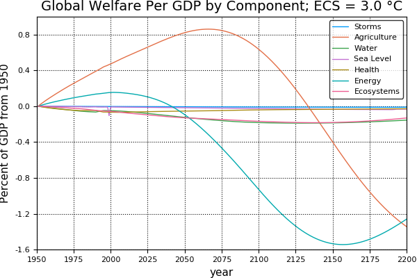
Figure 5.
FUND calculates, assuming an ECS of 3.0 °C and CO2 emissions increase to 89.2 GtCO2 by 2100, that the global storm damages change from 1950 to the year 2100 are 0.0090% of GDP, which is very insignificant.
Storms have always occurred, and they are not getting more frequent nor significantly more severe. Globally, weather-related monetary losses have decreased by about 25% since 1990 as a proportion of GDP. We should continue to improve our buildings and infrastructure to withstand severe storms to the extent where practical, but we should not blame CO2 emissions for causing more severe storms.
~~~~
Ken Gregory, B.AppSc., President of Friends of Science
Some of the curves on figures 4 and 5 may be difficult to identify. I made the curves thin to minimized the curve overlap. A person made a comment on Twitter “Interesting to look at the impact of Drought though. Cost is nearly $100 billion in 2016”. This is incorrect. The drought impact, identified as “Water” in the legend, from 1950 to 2016 is -$30 billion in figure 4 and -$49 billion is figure 5. The corresponding impact per GDP is -0.041% in figure 4 and -0.067% in figure 5. The writer might have confused the energy and water curves. The energy impact from 1950 to 2016 is +$104 billion in figure 4 and +$100 billion in figure 5.
To assist in identifying the curves, the values of each impact in the year 2100 relative to 2015 as GDP% in Figure 4 are;
Storms -0.0046%
Agriculture +1.202%
Water -0.093%
Sea Level -0.012%
Health -0.019%
Energy -0.115%
Ecosystems -0.099%
Oops, the previous sentence should be “To assist in identifying the curves, the values of each impact in the year 2100 relative to 1950 as GDP% in Figure 4 are;