Calculating the “Social Cost” of CO2 Emissions Using FUND*
(*The Climate Framework for Uncertainty, Negotiation and Distribution – an Integrated Economic Assessment Model)
Contributed by Ian Cameron © 2017
Introduction
Government agencies, such as Environment and Climate Change Canada (EC), define the social cost of CO2 or SCCO2 (more commonly misstated as the “social cost of carbon” or SCC) as “… an estimate of the monetary value in a given year of worldwide damage that will occur over the coming decades and centuries from emitting one additional tonne of CO2 emissions.” [EC’s March 2016 Technical Update to Social Cost of Greenhouse Gas Estimates, p. 1.] In other words, the agencies assume that any incremental emissions of CO2 are going to increase global temperatures for a number of years, thus causing general harm (in economists’ terminology, a global public “bad”) for as long the emissions remain in the atmosphere.
A typical use for SCCO2 is in policy analysis, such as doing cost-benefit calculations for proposed government regulations. For example, the EC Technical Update, p.i, states: “Estimates of the SCC therefore provide a way to value CO2 emission changes in cost- benefit analysis where the goal is to provide informed analysis to decision makers that quantifies the incremental mitigation benefits associated with a policy action and compares them to the incremental costs of abatement.” That is, the bureaucrats use the calculated SCCO2 to convince political leaders to impose greenhouse-gas reduction policies on their citizens.
According to the Technical Update EC relies for its SCCO2 estimates on the work of the US Interagency Working Group on the Social Cost of Carbon/Greenhouse Gases (IWG), which published its own technical update in August 2016. The IWG results are in US dollars, which EC converted to Canadian. To calculate the SCCO2 the IWG used three integrated assessment models (IAMs) called DICE (Dynamic Integrated Climate and Energy), FUND (Climate Framework for Uncertainty, Negotiation and Distribution) and PAGE (Policy Analysis of the Greenhouse Effect). As explained on page 15 of the Technical Update the IWG averaged results from the three models with five socioeconomic emissions scenarios using three discount rates (2.5, 3 and 5%) to reduce a series to future costs to one number (the SCCO2).
IAMS differ from the general circulation climate models (GCMs) in that they consider demographic, ecological, political and economic variables in addition to the physical climate system. GCMs employ complex mathematical models of the circulation of the Earth’s atmosphere and oceans in a three-dimensional grid, stepping forward in time. One of the outputs from the GCMs is future global temperatures, from which it is possible to calculate equilibrium climate sensitivities (ECS) – the eventual temperature rise in °C resulting from a doubling of atmospheric CO2 concentration. IAMs take these ECS (or rather a probabilistic range of ECS) to calculate future changes in global temperatures, from which they determine the resulting impacts on, for example, regional temperatures, sea-level rise, storms, land loss, agriculture, forests, water resources, biodiversity, human health and income.
Equilibrium Climate Sensitivity
The ECS supplied with FUND is a truncated gamma probability distribution, as shown in Figure 1. It has a minimum value of 1.0°C, peaks at 3.0°C (the statistical mode) and has a long tail extending to the right, theoretically to infinity. Because of the curve is skewed to the right, the average ECS is 3.5°C (which divides the area under the curve into equal parts.) The reason for this ECS distribution is found in an entry on Judith Curry’s blog describing a recent paper published by her and Nicholas Lewis. The blog entry contains excerpts from the IPCC’s AR5 report where the IPCC concluded: “Equilibrium climate sensitivity is likely in the range 1.5°C to 4.5°C (high confidence), extremely unlikely less than 1°C (high confidence), and very unlikely greater than 6°C (medium confidence).” Hence, the skewed curve, with a minimum of 1.0°C, shown in Figure 1.
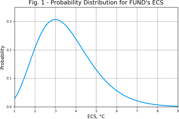
The Lewis and Curry paper relied on comprehensive 1750-2011 time series and uncertainty ranges for climate forcing components, together with estimates of heat accumulation in the climate system. That is, the authors used climate records, rather than GCMs, arriving at a median estimate for ECS of 1.64°C. Later Dr. Lewis reduced his ECS to 1.45°C by using new aerosol estimates, but even this failed to account for natural climate change (the millennium cycle recovery from the Little Ice Age) and the urban heat island effect. Adjusting for these factors gives an ESC best estimate of 1.02°C. Therefore, the following SCC calculations use ECS values of 3.5°C and 1.0°C.
Accessing FUND
Because they rely on an input ECS, IAMs use simple calculations to determine temperature as a function of atmospheric greenhouse gas concentrations and can run on desktop computers, rather than the supercomputers needed for the GCMs. One of the IAMs, FUND, is freely available for download and use by anyone with coding skills and some knowledge of the Julia language (to study the FUND code and then use it for calculations and analysis). FUND’s home page contains additional information and references to various publications that relied on the model.
FUND divides the world into 16 regions: USA, Canada, Western Europe, Japan-Korea, Australia-New Zealand, Eastern Europe, Former Soviet Union, Middle East, Central America, Latin America, South Asia, South-East Asia, China, North Africa, Sub-Saharan Africa and Small Island States. Each region may have its own input parameters by year (e.g., for population and economic growth rates), while some parameters are global in nature (e.g., ECS). The model calculates a global temperature change for each year from which it determines temperature changes for each of the regions. The effects of these changes, as well as sea-level rise, have economic and environmental effects on each region, including forced migrations among the regions.
The Appendix to this report lists the 29 components making up the FUND model, together with each component’s incoming parameters and outgoing variables.
The following plots and table give some idea of what FUND does. It starts in 1950 (the1950-2000 period is used to calibrate the model) and runs in one-year time-steps to 3000. However, the IWG and EC use 2300 as the end year for their SCCO2 calculations. They also have five socioeconomic scenarios called Base, Image, Merge, Message and MiniCAM. Page 7 of the EC Technical Update mentions the last four, and the Base scenario appears to be a business-as-usual case. The IPCC’s website also discusses the scenarios. The scenarios differ only in six input parameters: methane emissions; nitrous oxide emissions; carbon efficiency improvement indices; energy efficiency improvement indices; population growth rates; and economic growth rates.
FUND has 201 files of data of input parameters. Of these, 106 contain fixed values and the remaining 95 have probability distributions of either normal, triangular or gamma types. The latter includes the ECS. For a given scenario and several years of CO2 emission, the IWG ran FUND and the other two IAMs 10,000 times with random draws for the ECS and other probability distributions, then averaged the resulting SCCO2 values for all three models and scenarios. See pages 3 and 4 of the EC Technical Update for a more complete description of the process.
FUND Results
The results discussed below come from single runs of FUND using two values of ECS and the mode (most probable value) for all the other probability distributions.
Figure 2 shows global populations for the five scenarios. These curves are the result of the population growth-rate inputs, less deaths from normal mortality as well as from climate change effects (disease, storms, etc.)

Figures 3 and 4 depict the annual CO2 emissions and resulting atmospheric concentrations. There is a time lag between when emissions and concentrations peak because of CO2 persistence in the atmosphere.

Figures 5 and 6 show the sea-level and temperature rises assuming an ECS of 3.5°C, while Figures 7 and 8 present the results for a more reasonable ECS of 1.0°C. The calculations behind these curves are quite simple. For example, FUND’s climate forcing component requires 7 lines of code to determine the radiative forcing (in W/m2) from atmospheric greenhouse gas concentrations (CO2, as well as methane, nitrous oxide and sulfur hexafluoride) and the climate dynamics component has another 5 lines to calculate the temperature change resulting from the radiative forcing and ECS. The oceans component uses 2 lines of code to calculate the sea-level rise based on temperature. Both the climate dynamics and ocean components also incorporate time delays and various constants in their calculations.
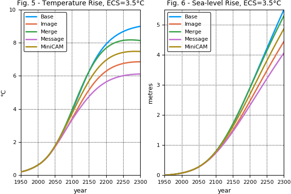
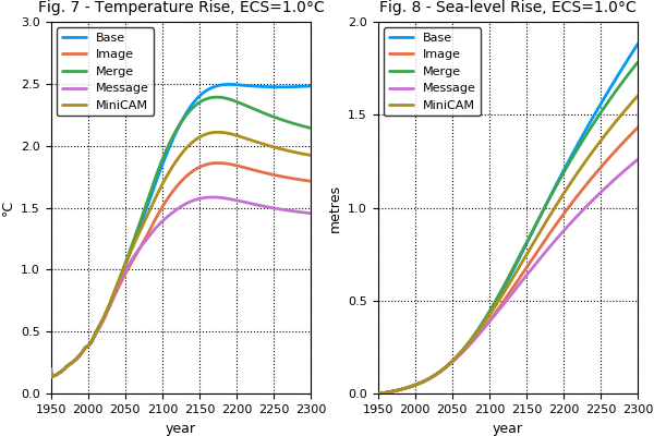
In Figures 7 and 8 the lower ECS reduces the temperature and sea-level rises by approximately the ratio of the two ECS values.
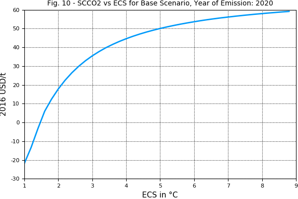
FUND calculates the annual global costs associated with a one-tonne release of a greenhouse gas in any given year. Figure 9 plots these costs for 1 t of CO2 released in 2020 in the Base scenario for ECS of 3.5°C and 1.0°C.

Both curves show sharp positive and negative changes in the initial years (2018-2030). For the ECS = 3.5°C plot there are some sharp negative spikes in about 2190, 2230 and 2270. These all result from the fact that FUND calculates marginal damages for each of the 16 regions and adds them to get a global total for each year. Sudden year-to-year changes in one or more regions can make a noticeable difference to the global total and the otherwise smooth curves in Figure 9. In the initial years, Western Europe, Japan-Korea, and China regions are responsible for the negative global values. For the ECS = 3.5°C, the USA region causes the negative spike near 2190; in 2230 it’s Central America, and in 2270 it’s South Asia.
In calculating regional damages from global warming FUND evaluates the various costs listed as inputs to Component 29 in the Appendix. As a result, the overall results in a given year are subject to sudden changes in any of these inputs.
However, the prime use of FUND is to calculate SCCO2. Table 1 shows the results for the Base scenario, using a 3% discount rate.
Table 1 – Calculated Social Costs of CO2 Emitted in Various Years (2016 $US/t)
| Emission Year | ECS = 3.5°C | ECS = 1.0°C |
| 2010 | 30 | -16 |
| 2020 | 41 | -22 |
| 2030 | 58 | -30 |
| 2040 | 86 | -28 |
| 2050 | 117 | -26 |
For an ECS of 3.5°C the calculated SCCO2 values increase significantly with the year of emission. This gives governments justification for steadily increasing carbon taxes (or cost of emissions permits under cap-and-trade schemes.) For an ECS of 1.0°C all the SCCO2 values are negative. In other words emissions of CO2 produce a net benefit to the world. This is in spite of the fact that (in Figure 7) global temperature increases well beyond the 2.0°C limit set by the UN Framework Convention on Climate Change. (Google “2.0°C limit” and you’ll get numerous links to articles affirming how bad it is.)
Figure 10 plots SCCO2 vs ECS for emission year 2020, showing that an ECS of about 1.5°C is the break-even value.
Conclusions
Ross McKitrick, who knows something about economic models, wrote a newspaper article for the National Post’s Junk Science Week series about the IAMs. Regarding FUND, PAGE and DICE he said: “They still all rely on simplified representations of the economy and the climate. And, most importantly, they all depend heavily on a handful of guesstimates on key parameters.” He also made this observation about FUND: “FUND differs from the other two IAMs because it takes into account CO2 fertilization of plants and the observation that moderate warming in some regions will be a net benefit. The other models assume that all CO2 is bad and any temperature change (up or down) is bad, which are themselves assumptions worthy of being challenged.”
Dr. McKitrick concluded: “The numbers produced by the IWG have a large and growing influence over energy and economic policy in the U.S. and Canada and elsewhere. Unfortunately, for all its claims about following the science, where it really counts it ended up peddling guesstimates based on inconsistent models. To borrow a phrase, it is time to restore science to its rightful place. Calculations behind the social cost of carbon need to reflect empirical evidence about low climate sensitivity, and when this is done, the numbers appear to be much lower than those currently in use.”
Dr. McKitrick isn’t the only economist critical of the IAMs. Patrick Michaels of the Cato Institute prepared some slides for a presentation on the subject of SCC. The slides discuss ECS, CO2 fertilization, domestic vs global SCC, choice of discount rates, and end with a quote from MIT economist Robert Pindyck: “An IAM-based analysis suggests a level of knowledge and precision that is nonexistent, and allows the modeler to obtain almost any desired result because key inputs can be chosen arbitrarily.”
Finally, the IWG, upon which EC has been relying for its SCCO2 calculations no longer exists. Last March President Trump signed an executive order to disband it. The next time EC updates its SCCO2 estimates, it will have to do so on its own.
The Julia code for producing the graphs is here.
Appendix – FUND’s Component Connections
The following list shows the 29 FUND components, together with each component’s incoming parameters and outgoing variables. These variables then become parameters for other components further down the list as FUND processes the list during each time-step. The names of most of the components, parameters and variables are obvious from their context, but some are cryptic. At the end of the component list is a table of the cryptic symbols.
1. scenariouncertainty component
incoming parameters:
none
outgoing variables:
– pgrowth in population component
– pgrowth in socioeconomic component
– ypcgrowth in socioeconomic component
– forestemm in emissions component
– aeei in emissions component
– acei in emissions component
– ypcgrowth in emissions component
- population component
incoming parameters:
– pgrowth from scenariouncertainty component
– enter from impactsealevelrise component
– leave from impactsealevelrise component
– dead from impactdeathmorbidity component
outgoing variables:
– globalpopulation in socioeconomic component
– populationin1 in socioeconomic component
– population in socioeconomic component
– population in emissions component
– population in impactagriculture component
– population in impactbiodiversity component
– population in impactcardiovascularrespiratory component
– population in impactcooling component
– population in impactdiarrhoea component
– population in impactextratropicalstorms component
– population in impactforests component
– population in impactheating component
– population in impactvectorbornediseases component
– population in impacttropicalstorms component
– population in vslvmorb component
– population in impactdeathmorbidity component
– population in impactwaterresources component
– population in impactsealevelrise component
- geography component
incoming parameters:
– landloss from impactsealevelrise component
outgoing variables:
– area in socioeconomic component
– area in impactsealevelrise component
- socioeconomic component
incoming parameters:
– area from geography component
– globalpopulation from population component
– populationin1 from population component
– population from population component
– pgrowth from scenariouncertainty component
– ypcgrowth from scenariouncertainty component
– eloss from impactaggregation component
– sloss from impactaggregation component
– mitigationcost from emissions component
outgoing variables:
– income in emissions component
– income in impactagriculture component
– income in impactbiodiversity component
– plus in impactcardiovascularrespiratory component
– urbpop in impactcardiovascularrespiratory component
– income in impactcooling component
– income in impactdiarrhoea component
– income in impactextratropicalstorms component
– income in impactforests component
– income in impactheating component
– income in impactvectorbornediseases component
– income in impacttropicalstorms component
– income in vslvmorb component
– income in impactwaterresources component
– income in impactsealevelrise component
– income in impactaggregation component
- emissions component
incoming parameters:
– income from socioeconomic component
– population from population component
– forestemm from scenariouncertainty component
– aeei from scenariouncertainty component
– acei from scenariouncertainty component
– ypcgrowth from scenariouncertainty component
outgoing variables:
– mitigationcost in socioeconomic component
– mco2 in climateco2cycle component
– globch4 in climatech4cycle component
– globn2o in climaten2ocycle component
– globsf6 in climatesf6cycle component
– cumaeei in impactcooling component
– cumaeei in impactheating component
- climateco2cycle component
incoming parameters:
– mco2 from emissions component
– temp from climatedynamics component
outgoing variables:
– acco2 in climateforcing component
– acco2 in impactagriculture component
– acco2 in impactextratropicalstorms component
– acco2 in impactforests component
- climatech4cycle component
incoming parameters:
– globch4 from emissions component
outgoing variables:
– acch4 in climateforcing component
- climaten2ocycle component
incoming parameters:
– globn2o from emissions component
outgoing variables:
– acn2o in climateforcing component
- climatesf6cycle component
incoming parameters:
– globsf6 from emissions component
outgoing variables:
– acsf6 in climateforcing component
- climateforcing component
incoming parameters:
– acco2 from climateco2cycle component
– acch4 from climatech4cycle component
– acn2o from climaten2ocycle component
– acsf6 from climatesf6cycle component
outgoing variables:
– radforc in climatedynamics component
- climatedynamics component
incoming parameters:
– radforc from climateforcing component
outgoing variables: – temp in climateco2cycle component
– temp in climateregional component
– temp in biodiversity component
– temp in ocean component
- biodiversity component
incoming parameters:
– temp from climatedynamics component
outgoing variables:
– nospecies in impactbiodiversity component
- climateregional component
incoming parameters:
– inputtemp from climatedynamics component
outgoing variables:
– temp in impactagriculture component
– temp in impactbiodiversity component
– temp in impactcardiovascularrespiratory component
– temp in impactcooling component
– regtmp in impactdiarrhoea component
– temp in impactforests component
– temp in impactheating component
– temp in impactvectorbornediseases component
– regstmp in impacttropicalstorms component
– temp in impactwaterresources component
- ocean component
incoming parameters:
– temp from climatedynamics component
outgoing variables:
– sea in impactsealevelrise component
- impactagriculture component
incoming parameters:
– population from population component
– income from socioeconomic component
– temp from climateregional component
– acco2 from climateco2cycle component
outgoing variables:
– agcost in impactaggregation component
- impactbiodiversity component
incoming parameters:
– temp from climateregional component
– nospecies from biodiversity component
– income from socioeconomic component
– population from population component
outgoing variables:
– species in impactaggregation component
- impactcardiovascularrespiratory component
incoming parameters:
– population from population component
– temp from climateregional component
– plus from socioeconomic component
– urbpop from socioeconomic component
outgoing variables:
– cardheat in impactdeathmorbidity component
– cardcold in impactdeathmorbidity component
– resp in impactdeathmorbidity component
- impactcooling component
incoming parameters:
– population from population component
– income from socioeconomic component
– temp from climateregional component
– cumaeei from emissions component
outgoing variables
– cooling in impactaggregation component
- impactdiarrhoea component
incoming parameters:
– population from population component
– income from socioeconomic component
– regtmp from climateregional component
outgoing variables:
– diadead in impactdeathmorbidity component
– diasick in impactdeathmorbidity component
- impactextratropicalstorms component
incoming parameters:
– population from population component
– income from socioeconomic component
– acco2 from climateco2cycle component
outgoing variables:
– extratropicalstormsdead in impactdeathmorbidity component
– extratropicalstormsdam in impactaggregation component
- impactforests component
incoming parameters:
– population from population component
– income from socioeconomic component
– temp from climateregional component
– acco2 from climateco2cycle component
outgoing variables:
– forests in impactaggregation component
- impactheating component
incoming parameters:
– population from population component
– income from socioeconomic component
– temp from climateregional component
– cumaeei from emissions component
outgoing variables:
– heating in impactaggregation component
- impactvectorbornediseases component
incoming parameters:
– population from population component
– income from socioeconomic component
– temp from climateregional component
outgoing variables:
– dengue in impactdeathmorbidity component
– schisto in impactdeathmorbidity component
– malaria in impactdeathmorbidity component
- impacttropicalstorms component
incoming parameters:
– population from population component
– income from socioeconomic component
– regstmp from climateregional component
outgoing variables:
– hurrdead in impactdeathmorbidity component
– hurrdam in impactaggregation component
- vslvmorb component
incoming parameters:
– population from population component
– income from socioeconomic component
outgoing variables
– vsl in impactdeathmorbidity component
– vmorb in impactdeathmorbidity component
- impactdeathmorbidity component
incoming parameters:
– vsl from vslvmorb component
– vmorb from vslvmorb component
– population from population component
– dengue from impactvectorbornediseases component
– schisto from impactvectorbornediseases component
– malaria from impactvectorbornediseases component
– cardheat from impactcardiovascularrespiratory component
– cardcold from impactcardiovascularrespiratory component
– resp from impactcardiovascularrespiratory component
– diadead from impactdiarrhoea component
– hurrdead from impacttropicalstorms component
– extratropicalstormsdead from impactextratropicalstorms component
– diasick from impactdiarrhoea component
outgoing variables:
– dead in population component
– deadcost in impactaggregation component
– morbcost in impactaggregation component
- impactwaterresources component
incoming parameters:
– population from population component
– income from socioeconomic component
– temp from climateregional component
outgoing variables:
– water in impactaggregation component
- impactsealevelrise component
incoming parameters:
– population from population component
– income from socioeconomic component
– sea from ocean component
– area from geography component
outgoing variables:
– landloss in geography component
– enter in population component
– leave in population component
– drycost in impactaggregation component
– protcost in impactaggregation component
– entercost in impactaggregation component
– wetcost in impactaggregation component
– leavecost in impactaggregation component
- impactaggregation component
incoming parameters:
– income from socioeconomic component
– heating from impactheating component
– cooling from impactcooling component
– agcost from impactagriculture component
– species from impactbiodiversity component
– water from impactwaterresources component
– hurrdam from impacttropicalstorms component
– extratropicalstormsdam from impactextratropicalstorms component
– forests from impactforests component
– drycost from impactsealevelrise component
– protcost from impactsealevelrise component
– entercost from impactsealevelrise component
– deadcost from impactdeathmorbidity component
– morbcost from impactdeathmorbidity component
– wetcost from impactsealevelrise component
– leavecost from impactsealevelrise component
outgoing variables:
– eloss in socioeconomic component
– sloss in socioeconomic component
Table of Cryptic Symbols
| Symbol | Meaning |
| ypcgrowth | Per capita income growth |
| forestemm | Forestry emissions parameter |
| acei | Autonomous carbon efficiency improvement |
| aeei | Autonomous energy efficiency improvement |
| mco2 | Emissions of CO2 |
| acco2 | Atmospheric concentration of CO2 |
| pgrowth | Population growth |
| sloss | Non-economic losses (species, deaths, morbidity, wetlands, leaving) |
| eloss | Economic losses (water, forest, heating, cooling, agriculture, drylands, protection against sea-level rise, entering, hurricane damage, extra-tropical storms) |
| urbpop | Urban population |
| wetcost | Cost of wetlands |
| drycost | Cost of dryland |
| leavecost | Cost of migration from regions |
| entercost | Cost of migration into regions |
| protcost | Cost of mitigation against sea-level rise |

All based on climate sensitivity…
What value of climate sensitivity?
Here are some recent public measures of that elusive parameter, with TCS and ECR trends:
https://pbs.twimg.com/media/C4zzXOoVcAAC51w.jpg
https://landshape.wordpress.com/2015/06/20/6921/
It is interesting to speculate what will happen to the TCS and ECR trends if we extrapolate them out to around 2025-2030.